

Contributions From: Michael Arrington, Ninos Mansor, Ron Palmeri, Heather Harde
The contents of this report are the opinion of Arrington XRP Capital and do not constitute financial advice. We cannot guarantee the accuracy and completeness of the information contained herein.
Risk management frameworks are rare in the world of Bitcoin. For overexposed market participants, the asset’s volatility invites extremes in investor psychology at a pace unlike any other market. Somehow, Bitcoin continues to dance between two distinct worlds: today on the brink of a death spiral and tomorrow the future of currency destined for world reserve status.
Arguments for Bitcoin exposure stress its long run outperformance, yet often fail to address the concerns of the non crypto-native investor. Since inception, Bitcoin has outperformed virtually every other asset class. This outperformance is undeniable, point-blank. Still, traditional portfolio managers stick to their skeptical guns, cautious of a one-sided focus on returns when the answer to double digit drawdown is HODL.
In this piece, we attempt to build a framework for risk-adjusted Bitcoin investing. Our goal is to filter out the noise of investor psychology and find the nuances of Bitcoin risk and reward at different stages of the macro cycle. We do this through a simple rolling Sharpe Ratio that analyzes Bitcoin risk-adjusted returns over time.
Ultimately, we conclude that timing matters: while the individual investor may be satisfied with long-run outperformance, Bitcoin’s macro cycles urge further nuance. We find that historically, the trade following the Halving represented the most attractive risk-adjusted opportunity. As the next Halving is just around the corner, we briefly speculate on why this was the case.
Looking beyond returns: the Sharpe Ratio
For the professional money manager, Bitcoin’s systematic risks are daunting. How can a conservative PM embrace Bitcoin as part of a diversified portfolio given the frequency and severity of its drawdowns? Investors with personal savings and unconstrained time horizons seek comfort in the story of Bitcoin’s long-run outperformance. This is not enough for newcomers with fiduciary responsibility. For the traditional PM, every market risk represents redemption, career and reputational risk; and for this reason, we need a more serious understanding of Bitcoin’s relationship with drawdown.
Even if over 90% of all Bitcoin days are profitable, individual paths to profitability range from months (buying December 2018’s bottom) to years (buying the 2014 global top). This illustrates the concept of path dependence: while long term Bitcoin returns are disproportionately skewed to the upside, timing matters. Much like a call option, Bitcoin risk-adjusted returns rapidly decay or improve depending on market timing.
We look to the Sharpe Ratio to analyse the path dependence of Bitcoin returns. The Sharpe Ratio is a simple yet powerful metric, measuring the ratio of excess returns to excess return volatility:
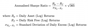
If we view volatility as a placeholder for risk, the Sharpe Ratio measures how much reward is generated per unit risk. A highly volatile portfolio would thus have a low Sharpe Ratio if returns were not extraordinary, and vice versa. A Sharpe Ratio of 1 is considered the baseline standard for investment performance.
Animal spirits, why a long-run Sharpe Ratio doesn’t cut it
Over any rolling four-year period, Bitcoin’s Sharpe Ratio historically outperformed virtually every other asset class. If an investor had held for at least four years during any point in Bitcoin’s history, they would have demonstrated superior risk-adjusted returns relative to almost all other investment opportunities.
This still falls short for most non crypto-native investors. Thinking about Bitcoin’s Sharpe Ratio over four year intervals may be correct in theory, but it is limited in practice. In reality, markets are governed by animal spirits – the swings of fear and greed – and most investors are more likely to enter the market after periods of non-linear growth. Many new entrants are thus destined to enter mid to late-cycle, fated to experience grueling drawdowns after buying local or even global highs. The assumption that investors can and will HODL underwater positions for multiple years is unfeasible, especially with the prospect of underperformance relative to other asset classes. The financial and emotional burden of drawdown will likely lead many to capitulate their positions before they are able to realise an entire four year cycle.
Given the path dependence of returns, the long term Sharpe Ratio fails to adequately capture Bitcoin risk.
The one year forward looking Sharpe Ratio
Instead of four-year intervals, we search for the optimal entry within a macro cycle. To do this, we employ a one year forward looking Sharpe Ratio.
Figure 1 calculates the Bitcoin Sharpe Ratio at any point in time looking forward one year. This metric is inherently forward looking, describing the Sharpe Ratio at any point in time based on future data. It is thus a lagging, descriptive (rather than predictive) variable. We select the one year period as it is approximately the time required to capture the brunt of a Bitcoin bull or bear market.

Oscillating around a value of 1, the one year forward looking Sharpe Ratio peaks at the beginning of Bitcoin’s price inception, the 2012 Halving and several months following the 2016 Halving. After these three periods, we find an interesting dynamic at play: aggressive Sharpe Ratio decay from a high of 3 (spectacular) to a low of −1 (abysmal).
Further, examining the 1-4 year forward looking Sharpe Ratio for Bitcoin from the Halvings (see Table 1), we find a similar effect:
- Exposure to Bitcoin for 1 year after the 2012 Halving nets a Sharpe Ratio of over 3, and holding for an additional 3 years degrades this to approximately 1. From a spectacular investment to a “good” investment.
- Exposure to Bitcoin for 1 year after the 2016 Halving nets a Sharpe Ratio of over 2, and holding for an additional 3 years degrades this to less than 1. From a great investment to a sub-standard investment.

How important is market timing when managing Bitcoin risk?
Analysing Sharpe Ratio decay gives us a powerful risk framework. Not all Bitcoin investments are made equal: Bitcoin acquired at different points in a macro cycle should be treated differently as part of a diversified portfolio. To illustrate this concept, consider the idea of “time-to-profitability” (TTP) demonstrated in Figure 2:
- Bitcoin acquired at the 2011 high has a ≈2 year TTP
- Bitcoin acquired at the late 2013 high has a ≈3 year TTP
- Bitcoin acquired at the 2017 high is yet to achieve profitability.

Not only were investors who purchased Bitcoin at these highs faced with absolute drawdown, they were also faced with relative underperformance against worldwide equity indices (and possibly other asset classes). Bitcoin can be an excellent tool within a diversified portfolio, but most professional investors cannot simply buy and HODL for extremely long periods of time if they are likely to face both absolute and relative underperformance.
The legacy wisdom of financial markets sometimes cautions investors against market timing, captured by the dominance of indexing strategies and the underwhelming reputation of the modern hedge fund. Whatever the merits of this argument in traditional markets, we find a fundamentally different heuristic exists for Bitcoin.
This doesn’t mean that other strategies like buy and HODL are not valid. It is simply to say that for investors focused on managing risk, timing matters.
A once-in-cycle trade, but don’t forget to expect the unexpected
The above analysis leads us to conclude that, historically, the best risk-adjusted entry existed at or within several months following a Bitcoin Halving. This heuristic is based on historical data and is not a trading guideline. The market may prove our analysis entirely wrong for future Halvings. Our goal is to build frameworks based on history but there are no certainties in markets, least of all in Bitcoin. We present this Halving idea with its obvious limitations in mind.
While the crypto market’s focus on long-run outperformance might convince some pioneering and brave money managers, it won’t convince the drawdown-conscious. However, Bitcoin doesn’t need to be perfect to make its way into the world of traditional investing. Even today, the argument shouldn’t be to HODL and hope, but to think about Bitcoin with a nuanced vision for risk. This post-Halving window, when combined with hedging practices like protective puts or a managed stop loss, help build a case that, on a risk-adjusted basis, Bitcoin may outperform other asset classes.
If Bitcoin springs to new highs within the next several years, the reality is that investors will eventually demand exposure. Ironically, as these requests pile in mid to late-cycle, money managers will be faced with a dicey dilemma: remain on zero as Bitcoin makes weekly headlines or enter a drawdown-prone asset at local or absolute highs. Rather than enter as greed floods the market, the post-Halving window may grant investors an early buffer to incorporate Bitcoin into their broader macro strategy.
Are there fundamentals that explain this finding?
Why does the Halving trade demonstrate superior risk-adjusted returns? We can only speculate, but PlanB’s Stock-To-Flow model provides some insight. If we slightly modify PlanB’s model to calculate “flow” as a rolling sum of new Bitcoin minted over the past year (as opposed to the past day), as per Figure 3, we find that the market tops as the S2F ratio begins to level off. This makes intuitive sense: assuming demand stays constant, the supply reduction means there is less float for buyers to absorb, shifting prices upwards over time until a new equilibrium is reached.
This could also explain why, in addition to the two Halvings, the early years following Bitcoin’s inception also represented a very strong risk-adjusted entry. With a low initial float (starting from S = 0 at launch), the 1-year S2F ratio grew at a rate comparable to the post-Halving windows.
We speculate that these periods of rising S2F following the Halving are the only times where there is a fundamental driver (outside of speculative demand) for Bitcoin price: a real shift in the supply and demand curve. Thus, it is possible that our conclusion about the Halving trade is not random, but a result of S2F fundamentals.

Conclusion
In this piece, we have shown that long term metrics such as the four year Sharpe Ratio are inadequate at capturing the real risks of Bitcoin investing. Extreme swings of the market result in rapid Sharpe Ratio decay and make timing critical for the drawdown-conscious investor. The post-Halving window may represent a rare time to add high expectancy, low-downside Bitcoin exposure. We hope that our analysis builds a case that the Halving is not merely a speculative catalyst, but a fundamental macro driver that may present crypto-natives and newcomers alike with a powerful risk-adjusted opportunity.